Neal’s funnel

Now lets take a distribution where a Gibbs sampler is needed to get a decent result, Neal’s funnel. In general Gibbs sampler is useful for hierarchical models, with each part of the hierarchy being treated as different steps.

import jax.numpy as jnp
import numpyro
import numpyro.distributions as dist
import arviz
import matplotlib.pyplot as plt

from numpyro.infer import MCMC, NUTS
from jax import random

from MultiHMCGibbs import MultiHMCGibbs

/opt/hostedtoolcache/Python/3.10.18/x64/lib/python3.10/site-packages/tqdm/auto.py:21: TqdmWarning: IProgress not found. Please update jupyter and ipywidgets. See https://ipywidgets.readthedocs.io/en/stable/user_install.html
  from .autonotebook import tqdm as notebook_tqdm

The model

We will set up 5 dimensional funnel, something that regular HMC struggles with. For this model we know what the true marginal distribution for the y variable will be Normal(0, 3), we will use this to see how well each sampler does.

def model(dim=5):
    y = numpyro.sample("y", dist.Normal(0, 3))
    numpyro.sample("x", dist.Normal(jnp.zeros(dim - 1), jnp.exp(y / 2)))


x_marginal_true = jnp.linspace(-10, 10, 1000)
y_marginal_true = jnp.exp(dist.Normal(0, 3).log_prob(x_marginal_true))

def run_inference(kernel, chain_method, rng_key):
    mcmc = MCMC(
        kernel,
        num_warmup=3000,
        num_samples=5000,
        num_chains=4,
        chain_method=chain_method,
        progress_bar=False
    )
    mcmc.run(rng_key)
    return mcmc

NUTS

We will use a large target_accept_prob to get rid of most divergent samples and use a large number of warmup and samples to get the r_hats close to 1.

rng_key = random.PRNGKey(0)
hmc_key, gibbs_key = random.split(rng_key)

funnel_mcmc_hmc = run_inference(NUTS(model, target_accept_prob=0.995), 'vectorized', hmc_key)
inf_funnel_hmc = arviz.from_numpyro(funnel_mcmc_hmc)
print(f'divergences per chain: {inf_funnel_hmc.sample_stats.diverging.values.sum(axis=1)}')
display(arviz.summary(inf_funnel_hmc))

divergences per chain: [  2   6 184  14]

	mean	sd	hdi_3%	hdi_97%	mcse_mean	mcse_sd	ess_bulk	ess_tail	r_hat
x[0]	-0.081	7.130	-7.619	6.867	0.125	1.159	11630.0	1546.0	1.05
x[1]	-0.133	6.629	-7.324	7.557	0.083	0.746	11451.0	1331.0	1.05
x[2]	0.075	8.082	-6.889	7.882	0.174	1.870	11027.0	1517.0	1.05
x[3]	-0.101	7.119	-7.190	7.732	0.108	0.989	13902.0	1363.0	1.05
y	-0.385	3.173	-6.504	4.674	0.508	0.335	44.0	27.0	1.07

Give the large number of divergent samples in chain 4 let’s remove that from the plots.

x_model_hmc = inf_funnel_hmc.isel(chain=[0, 1, 2]).posterior.x[..., 0].data.flatten()
y_model_hmc = inf_funnel_hmc.isel(chain=[0, 1, 2]).posterior.y.data.flatten()

plt.figure(figsize=(10, 4))
plt.subplot(121)
plt.plot(x_model_hmc, y_model_hmc, '.')
plt.xlabel('x[0]')
plt.ylabel('y')
plt.xlim(-100, 100)
plt.subplot(122)
plt.hist(y_model_hmc, bins=30, histtype='step', density=True, label='HMC')
plt.plot(x_marginal_true, y_marginal_true, color='k', label='True marginal')
plt.xlabel('y')
plt.legend();

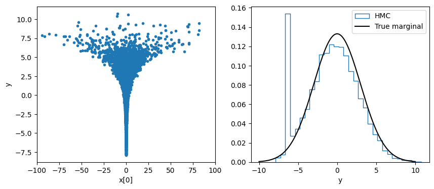
We can see that NUTS is struggling with this model, the y marginal is still missing a bit of negative values at the bottom of the funnel.

MultiHMCGibbs

For the MultiHMCGibbs sampler we will only put a large target_accept_prob on the x values (as these are the difficult ones to draw), but keep the default value for the y values. To keep it on the same footing as the previous run we will use the same number of warm up and sample draws.

funnel_mcmc_gibbs = run_inference(
    MultiHMCGibbs(
        [NUTS(model, target_accept_prob=0.995), NUTS(model)],
        [['x'], ['y']]
    ),
    'vectorized',
    gibbs_key
)
inf_funnel_gibbs = arviz.from_numpyro(funnel_mcmc_gibbs)
print(f'divergences per chain per step:\n {inf_funnel_gibbs.sample_stats.diverging.values.sum(axis=1).T}')
display(arviz.summary(inf_funnel_gibbs))

divergences per chain per step:
 [[  2  31   7 104]
 [  0   0   0   0]]

	mean	sd	hdi_3%	hdi_97%	mcse_mean	mcse_sd	ess_bulk	ess_tail	r_hat
x[0]	0.650	17.561	-10.245	9.306	0.776	5.492	6138.0	671.0	1.02
x[1]	-0.744	17.905	-9.776	9.957	1.000	6.168	4063.0	662.0	1.02
x[2]	-0.669	16.245	-9.097	10.016	0.583	4.933	6896.0	749.0	1.02
x[3]	-1.393	19.836	-9.993	10.110	1.371	7.707	3036.0	601.0	1.02
y	0.338	2.978	-5.338	5.596	0.186	0.136	268.0	339.0	1.02

Again chain 4 has a large number of divergences, so let’s remove it from the plots.

x_model_gibbs = inf_funnel_gibbs.isel(chain=[0, 1, 2]).posterior.x[..., 0].data.flatten()
y_model_gibbs = inf_funnel_gibbs.isel(chain=[0, 1, 2]).posterior.y.data.flatten()

plt.figure(figsize=(10, 4))
plt.subplot(121)
plt.plot(x_model_hmc, y_model_hmc, '.', label='HMC', zorder=2)
plt.plot(x_model_gibbs, y_model_gibbs, '.', label='Gibbs', zorder=1)
plt.xlabel('x[0]')
plt.ylabel('y')
plt.legend()
plt.xlim(-100, 100)
plt.subplot(122)
plt.hist(y_model_hmc, bins=30, histtype='step', label='HMC', density=True)
plt.hist(y_model_gibbs, bins=30, histtype='step', label='Gibbs', density=True)
plt.plot(x_marginal_true, y_marginal_true, color='k', label='True marginal')
plt.xlabel('y')
plt.legend();

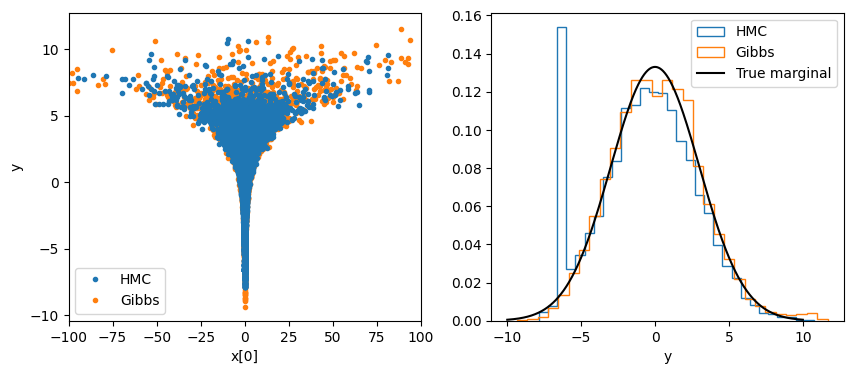
We can see that with the same set up MultiHMCGibbs was able to reach deeper into the funnel and pull out the negative y values missed by NUTS.

Note: Even if I did not remove chain 4 from both samples the results would be much the same. Under this parameterization this model is hard for both samplers to draw from, MultiHMCGibbs just does a better job with the same set up.

Other notes

• You can use as many inner_kernels as you want

• The order the kernels are stepped in is set by the order of the parameter list (in the example above x septs first, followed by y)

• The order matters! Typically you want to step the parameters closest to the likelihood first and the hyper-parameters second. But for some models this might not be so clear, so some experimentation could be needed.