Basic usage and comparison
This example will run through a basic comparison of MultiHMCGibbs with NUTS and HMCGibbs for a simple problem where all three methods should give the same results. Our target distribution will be a 2D normal with some covariance.
import jax.numpy as jnp
import numpyro
import numpyro.distributions as dist
import arviz
import corner
import matplotlib.pyplot as plt

from numpyro.infer import MCMC, NUTS, HMCGibbs
from jax import random

from MultiHMCGibbs import MultiHMCGibbs
/opt/hostedtoolcache/Python/3.10.19/x64/lib/python3.10/site-packages/tqdm/auto.py:21: TqdmWarning: IProgress not found. Please update jupyter and ipywidgets. See https://ipywidgets.readthedocs.io/en/stable/user_install.html
  from .autonotebook import tqdm as notebook_tqdm
/opt/hostedtoolcache/Python/3.10.19/x64/lib/python3.10/site-packages/arviz/__init__.py:39: FutureWarning:
ArviZ is undergoing a major refactor to improve flexibility and extensibility while maintaining a user-friendly interface.
Some upcoming changes may be backward incompatible.
For details and migration guidance, visit: https://python.arviz.org/en/latest/user_guide/migration_guide.html
  warn(
The model
As with any Numpyro sampler we start with a model function for our distribution.
def model():
    x = numpyro.sample("x", dist.Normal(0.0, 2.0))
    y = numpyro.sample("y", dist.Normal(0.0, 2.0))
    numpyro.sample("obs", dist.Normal(x + y, 1.0), obs=jnp.array([1.0]))
NUTS
To start we will use NUTS so we know what we are comparing to.
rng_key = random.PRNGKey(0)
hmc_key, rng_key = random.split(rng_key)
hmc_kernel = NUTS(model)
mcmc = MCMC(
    hmc_kernel,
    num_warmup=100,
    num_samples=1000,
    num_chains=4,
    chain_method='vectorized',
    progress_bar=False
)
mcmc.run(hmc_key)

inf_data_hmc = arviz.from_numpyro(mcmc)
print(f'divergences per chain: {inf_data_hmc.sample_stats.diverging.values.sum(axis=1)}')
display(arviz.summary(inf_data_hmc))
fig = corner.corner(inf_data_hmc, color='C0')
divergences per chain: [0 0 0 0]
| mean | sd | hdi_3% | hdi_97% | mcse_mean | mcse_sd | ess_bulk | ess_tail | r_hat | |
|---|---|---|---|---|---|---|---|---|---|
| x | 0.392 | 1.492 | -2.225 | 3.420 | 0.041 | 0.034 | 1308.0 | 1404.0 | 1.0 |
| y | 0.500 | 1.499 | -2.312 | 3.202 | 0.042 | 0.033 | 1281.0 | 1564.0 | 1.0 |

MultiHMCGibbs
To use MultiHMCGibbs you need to create a list of HMC or NUTS kernels that wrap the same model, but each can have their own keywords such as target_accept_prob or max_tree_depth. The other argument is a list of lists containing the free parameters for each of the inner kernels. Internally each the sampler will:
Loop over the kernels in the list
Conditioned it on the non-free parameters
Re-calculate the likelihood and gradients at the new conditioned point
Step the kernel forward
Move on to the next kernel
After stepping the last kernel all the parameters will be updated and a single Gibbs step has been taken.
Important: All free parameters must be listed exactly once for the sampler to work. If this is not the case a ValueError will be raised listing what values are either duplicated, extra, or missing from the list.
multigibbs_key, rng_key = random.split(rng_key)
inner_kernels = [
    NUTS(model),
    NUTS(model)
]

outer_kernel = MultiHMCGibbs(
    inner_kernels,
    [['y'], ['x']]  # first updated y, then update x
)

mcmc_gibbs = MCMC(
    outer_kernel,
    num_warmup=100,
    num_samples=1000,
    num_chains=4,
    chain_method='vectorized',
    progress_bar=False
)
mcmc_gibbs.run(multigibbs_key)

inf_data_gibbs = arviz.from_numpyro(mcmc_gibbs)
print(f'divergences per chain per step:\n {inf_data_gibbs.sample_stats.diverging.values.sum(axis=1).T}')
display(arviz.summary(inf_data_gibbs))

print('HMC (Blue)')
print('MultiHMCGibbs (Orange)')
fig = corner.corner(inf_data_gibbs, color='C1')
_ = corner.corner(inf_data_hmc, fig=fig, color='C0')
divergences per chain per step:
 [[0 0 0 0]
 [0 0 0 0]]
| mean | sd | hdi_3% | hdi_97% | mcse_mean | mcse_sd | ess_bulk | ess_tail | r_hat | |
|---|---|---|---|---|---|---|---|---|---|
| x | 0.337 | 1.515 | -2.704 | 2.994 | 0.085 | 0.045 | 319.0 | 611.0 | 1.02 |
| y | 0.549 | 1.514 | -2.211 | 3.332 | 0.091 | 0.044 | 277.0 | 689.0 | 1.02 |
HMC (Blue)
MultiHMCGibbs (Orange)
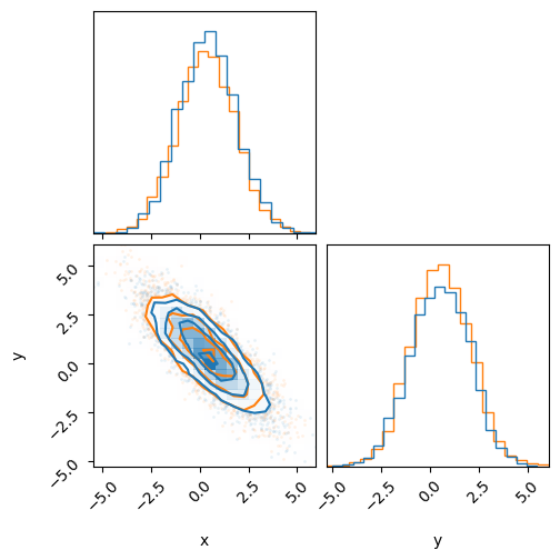
We can see that the two samplers give the same results, a good indication that everything is working.
HMCGibbs
For this simple model we can also do the conditioning on y by hand and use Numpyro’s builtin HMCGibbs sampler. Let’s see how that compares.
Note: We will use chian_method='sequential' for this sampler because it does support vectorized. We also don’t have access to the divergences of the HMC kernel so those will not be reported either.
gibbs_key, rng_key = random.split(rng_key)
def gibbs_fn(rng_key, gibbs_sites, hmc_sites):
    y = hmc_sites['y']
    new_x = dist.Normal(0.8 * (1-y), jnp.sqrt(0.8)).sample(rng_key)
    return {'x': new_x}


kernel_gibbs_fn = HMCGibbs(hmc_kernel, gibbs_fn=gibbs_fn, gibbs_sites=['x'])

mcmc_gibbs_fn = MCMC(
    kernel_gibbs_fn,
    num_warmup=100,
    num_samples=1000,
    num_chains=4,
    chain_method='sequential',
    progress_bar=False
)

mcmc_gibbs_fn.run(gibbs_key)

inf_data_gibbs_fn = arviz.from_numpyro(mcmc_gibbs_fn)
display(arviz.summary(inf_data_gibbs_fn))

print('HMC (Blue)')
print('MultiHMCGibbs (Orange)')
print('HMCGibbs (Green)')
fig = corner.corner(inf_data_gibbs, color='C1')
_ = corner.corner(inf_data_hmc, fig=fig, color='C0')
_ = corner.corner(inf_data_gibbs_fn, fig=fig, color='C2')
| mean | sd | hdi_3% | hdi_97% | mcse_mean | mcse_sd | ess_bulk | ess_tail | r_hat | |
|---|---|---|---|---|---|---|---|---|---|
| x | 0.425 | 1.441 | -2.260 | 3.145 | 0.058 | 0.026 | 623.0 | 1497.0 | 1.01 |
| y | 0.478 | 1.454 | -2.315 | 3.173 | 0.065 | 0.031 | 500.0 | 1083.0 | 1.01 |
HMC (Blue)
MultiHMCGibbs (Orange)
HMCGibbs (Green)

As before, we see that this sampler gives the same results.